ROS2 Development Walkthrough — BonicBot A2
Before you start: Make sure BonicBot A2 is powered on and you have a working terminal — either SSH’d into the robot, or inside the Docker dev container on your laptop.
Not set up yet? See the ROS2 Development Setup.
Part 1 — Drive the Robot with Your Keyboard
The first thing you should do with BonicBot A2 is move it. Everything else builds from here.
Make sure your laptop and the robot are on the same Wi-Fi network. ROS2 will discover the robot automatically — no extra configuration needed.
Launch Teleop
ros2 run teleop_twist_keyboard teleop_twist_keyboardClick on the terminal to give it focus, then drive:
| Key | Action |
|---|---|
i | Forward |
, | Backward |
j | Turn left |
l | Turn right |
k | Stop |
q / z | Faster / Slower |
Your keyboard is publishing velocity commands to the /cmd_vel topic. The robot’s motor controller is subscribed to it and responding in real time. That’s the ROS2 pub/sub model in action — and it works the same way whether you’re driving a real robot or a simulation.
Part 2 — Explore What the Robot is Doing
With the robot running, open a second terminal and start poking around.
List everything currently active:
ros2 topic list
ros2 node list
Stream live distance readings from the laser sensor:
ros2 topic echo /scanWatch the numbers change as you move objects near the robot. Each value is a real-time distance measurement from the robot’s surroundings. This is the same data that powers obstacle avoidance, SLAM, and autonomous navigation.
Try publishing a command directly without teleop:
ros2 topic pub /cmd_vel geometry_msgs/msg/Twist \
  "{linear: {x: 0.2}, angular: {z: 0.0}}"
The robot moves forward. You just sent a motion command from scratch — no driver code, no SDK. This is how ROS2 works at its core.
Part 3 — Visualise the Robot with RViz2
Show RViz2 setup steps
RViz2 gives you a live 3D view of the robot — its model, transforms, and sensor data — all updating as it moves.
RViz2 runs on your laptop. You need the Docker dev environment for this.
If you haven’t set it up: ROS2 Development Setup → Docker.
Launch RViz:
rvizIf the grid doesn’t appear, run this first:
echo "export LIBGL_ALWAYS_SOFTWARE=1" >> ~/.bashrc && source ~/.bashrcConfigure the display:
-
Change Fixed Frame from
map→odom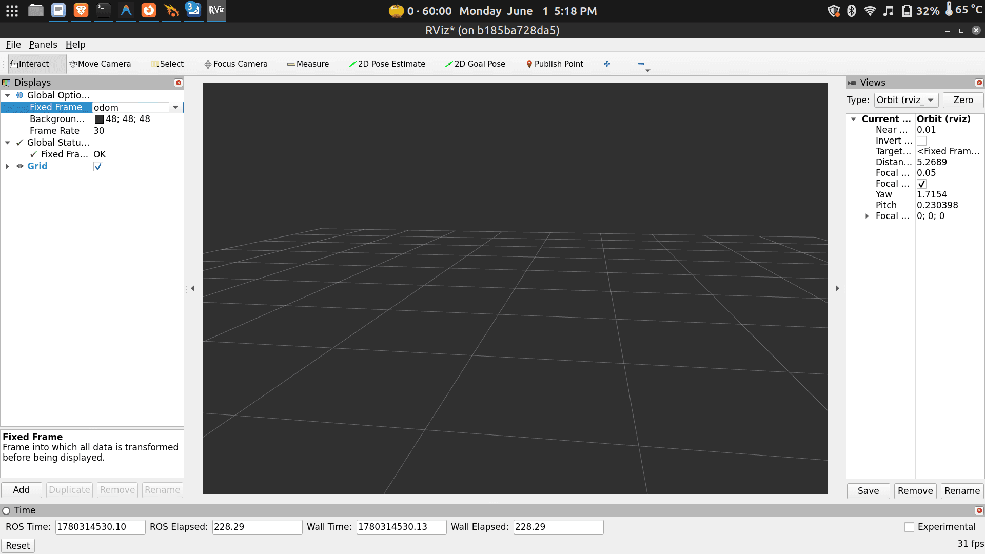
-
Click Add → select TF and RobotModel
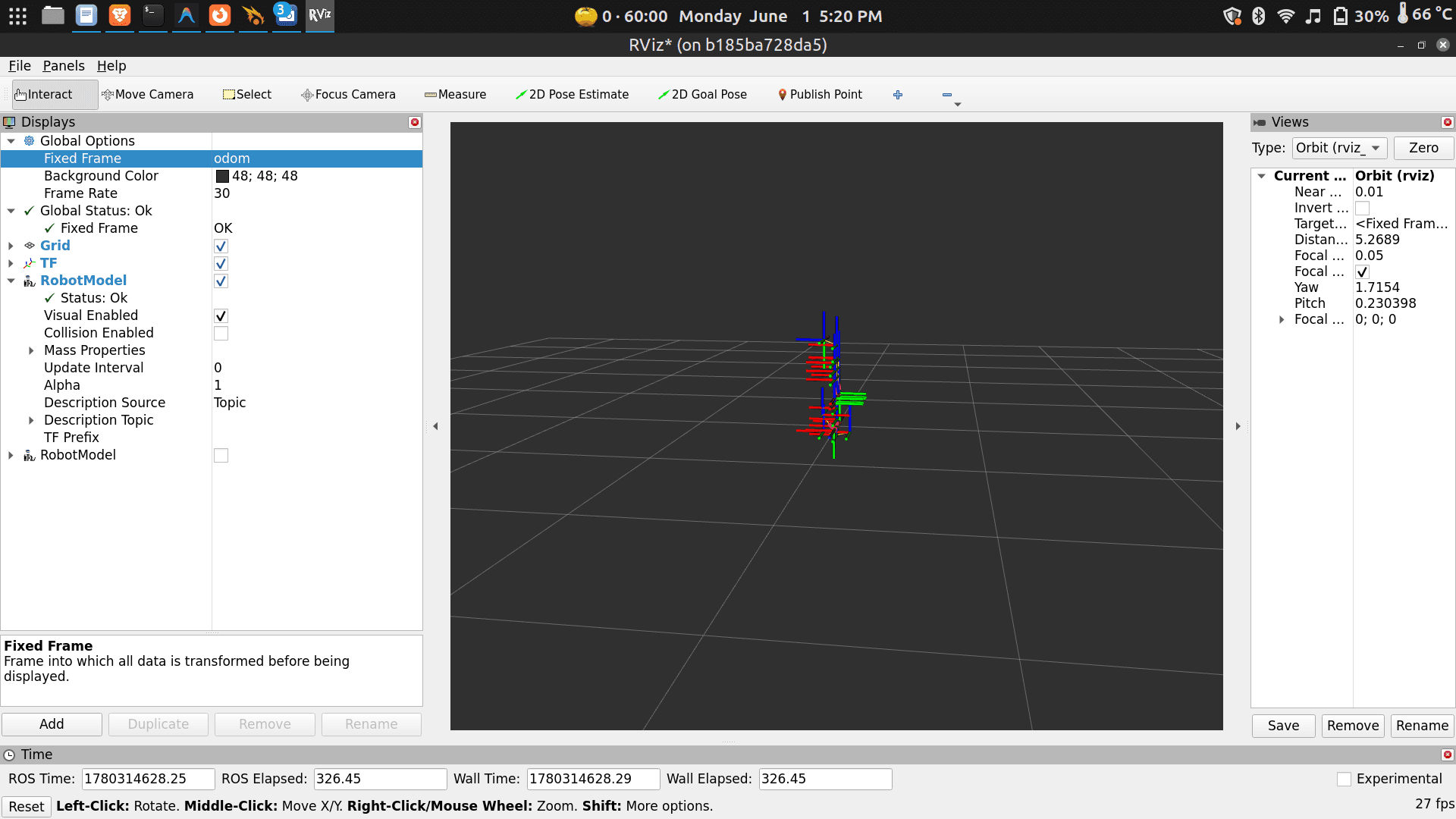
- Set Description Topic to
/robot_description
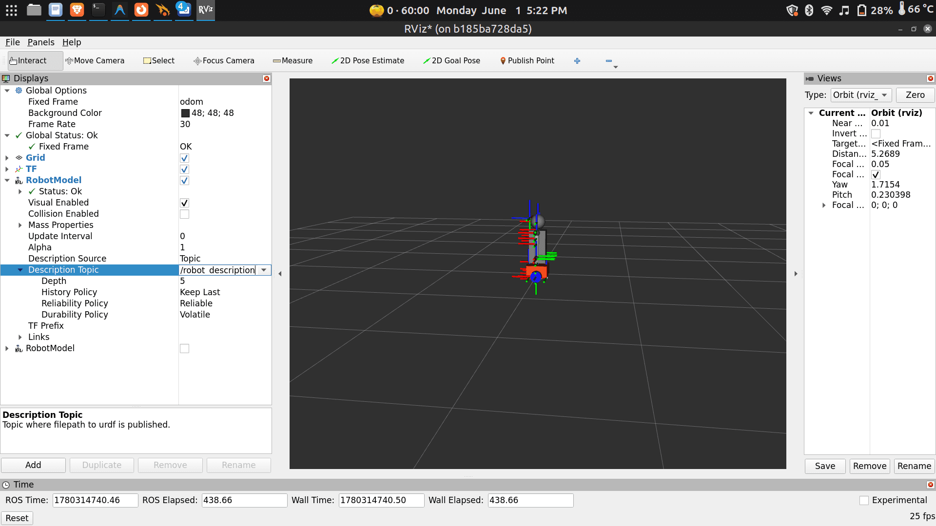
- Set Description Topic to
-
Click Add → select LaserScan
- Set Topic to
/scan - Set Size to
0.04for better visibility
 Now drive the robot with teleop in another terminal. Watch the laser scan sweep in real time as the robot turns and navigates.
 - Set Topic to
Part 4 — Run the Robot in Simulation
Don’t have the robot with you? Want to test code before running it on hardware? Gazebo gives you a virtual BonicBot A2 that behaves identically — same topics, same commands, same everything.
You need the Docker dev environment for this part. See ROS2 Development Setup → Docker.
First time — clone and build the workspace
⚠️ Do this once only.
mkdir -p ~/dev_ws/src
cd ~/dev_ws/src
git clone https://github.com/Autobonics/bonicbot-a2-ros.git
cd ~/dev_ws
colcon build --symlink-install
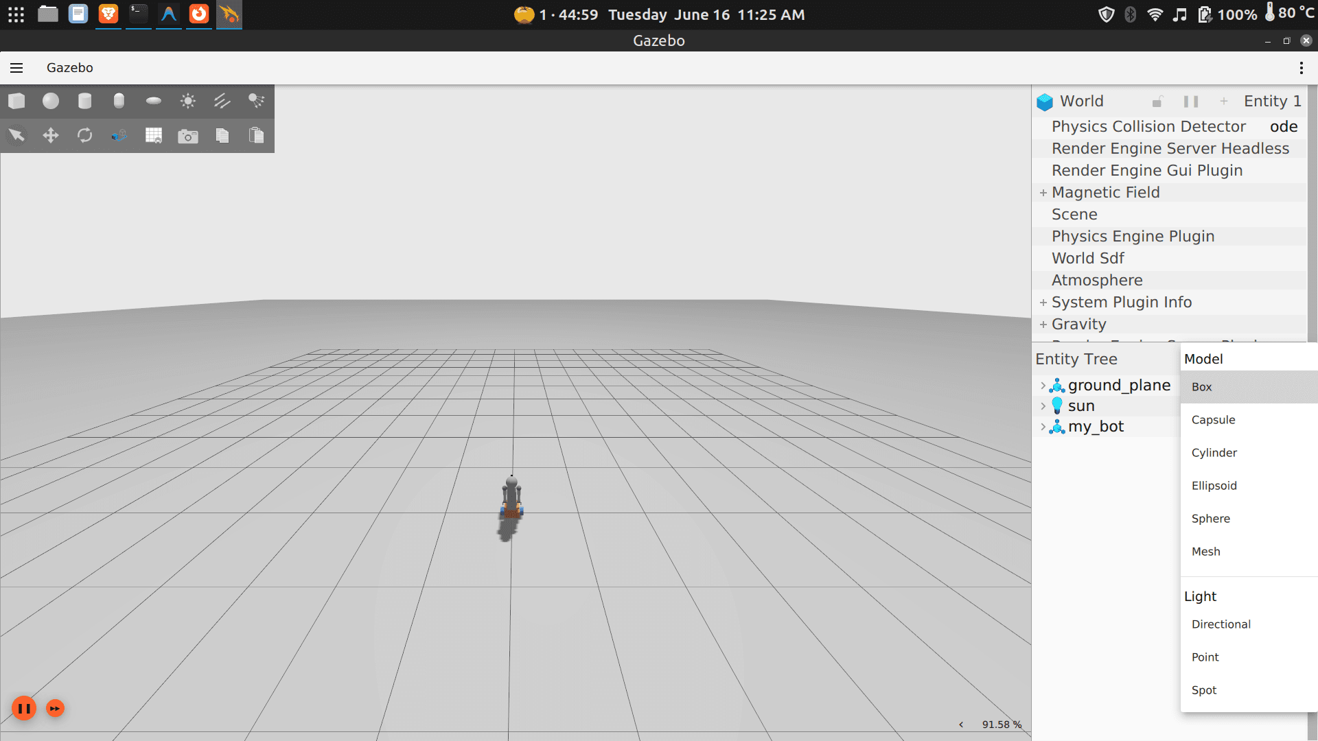
source install/setup.bashLaunch Gazebo
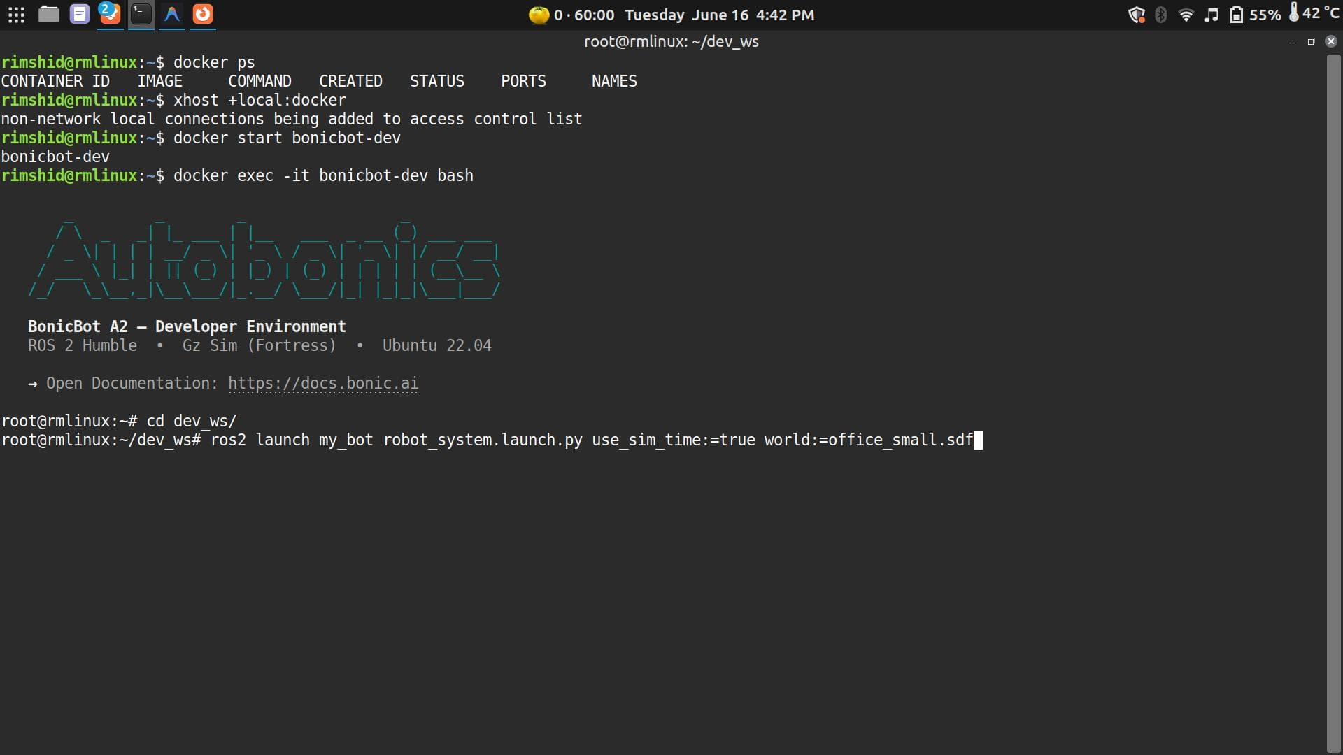
gazeboOr explicitly:
ros2 launch my_bot robot_system.launch.py use_sim_time:=trueTeleop in simulation
Open a second terminal and run teleop exactly as in Part 1:
cd ~/dev_ws && source install/setup.bash
ros2 run teleop_twist_keyboard teleop_twist_keyboard
Same command. Same topics. The only difference is what’s listening on the other end.
Next time you open this
docker start bonicbot-dev
docker exec -it bonicbot-dev bash
gazebo
Running BonicBot A2 in a Custom World
Show walkthrough
Once you can run the robot in simulation, the next step is building environments for it to navigate — spaces that mimic real rooms, corridors, and facilities — and running all your ROS2 workflows inside them. This is how robotics engineers prototype navigation, test code safely, and iterate quickly before touching real hardware.
Real Environment → Simulated Environment
The goal isn’t photorealism — it’s a space where the robot can sense obstacles, navigate, and behave the way it would in the physical world.
Real Environment
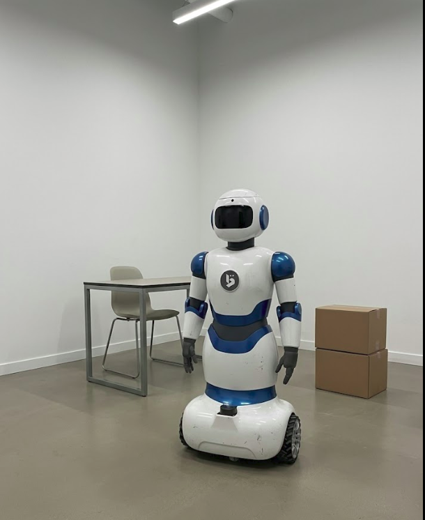
Walls become simple geometry, furniture becomes collision objects, and navigation spaces stay preserved. That’s enough for the robot’s lidar and physics to behave realistically.
Understanding the Gazebo Interface
Gazebo is both a robotics simulator and a 3D environment editor. You can insert objects, move obstacles, test robot behaviour, and build custom worlds — all from the same UI.
Creating a Custom World
By default, Gazebo loads an empty world — flat ground, no obstacles, nothing for your robot to interact with. A custom world is an environment you define: a room, a warehouse, an office corridor, a hospital ward. You place the walls, furniture, and objects. You decide the layout.
This matters because a robot doesn’t just need to move — it needs to move through something. Custom worlds let you:
- Test navigation — can the robot plan a path through a cluttered room?
- Simulate real spaces — replicate your actual environment before deploying
- Stress-test sensors — make sure the lidar, cameras, and depth sensors respond correctly to your specific layout
- Iterate safely — break things in simulation before touching real hardware
Every Gazebo world is stored as an SDF file (Simulation Description Format) — a text file that describes your environment’s geometry, objects, and physics. You don’t need to understand the file format to get started — the options below handle that for you.
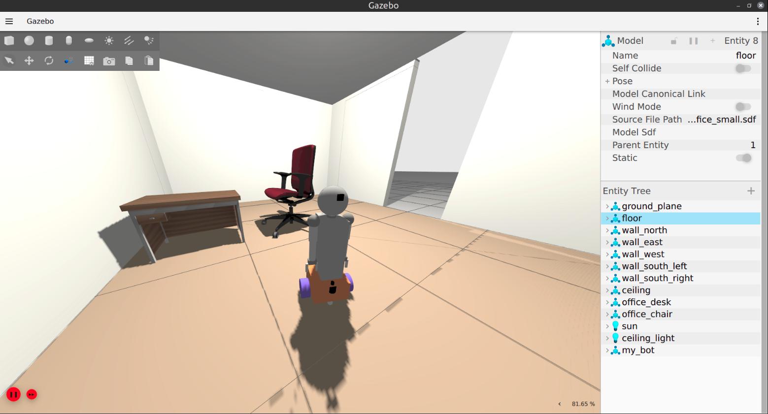
Option 1 — Build Your World Visually in Gazebo
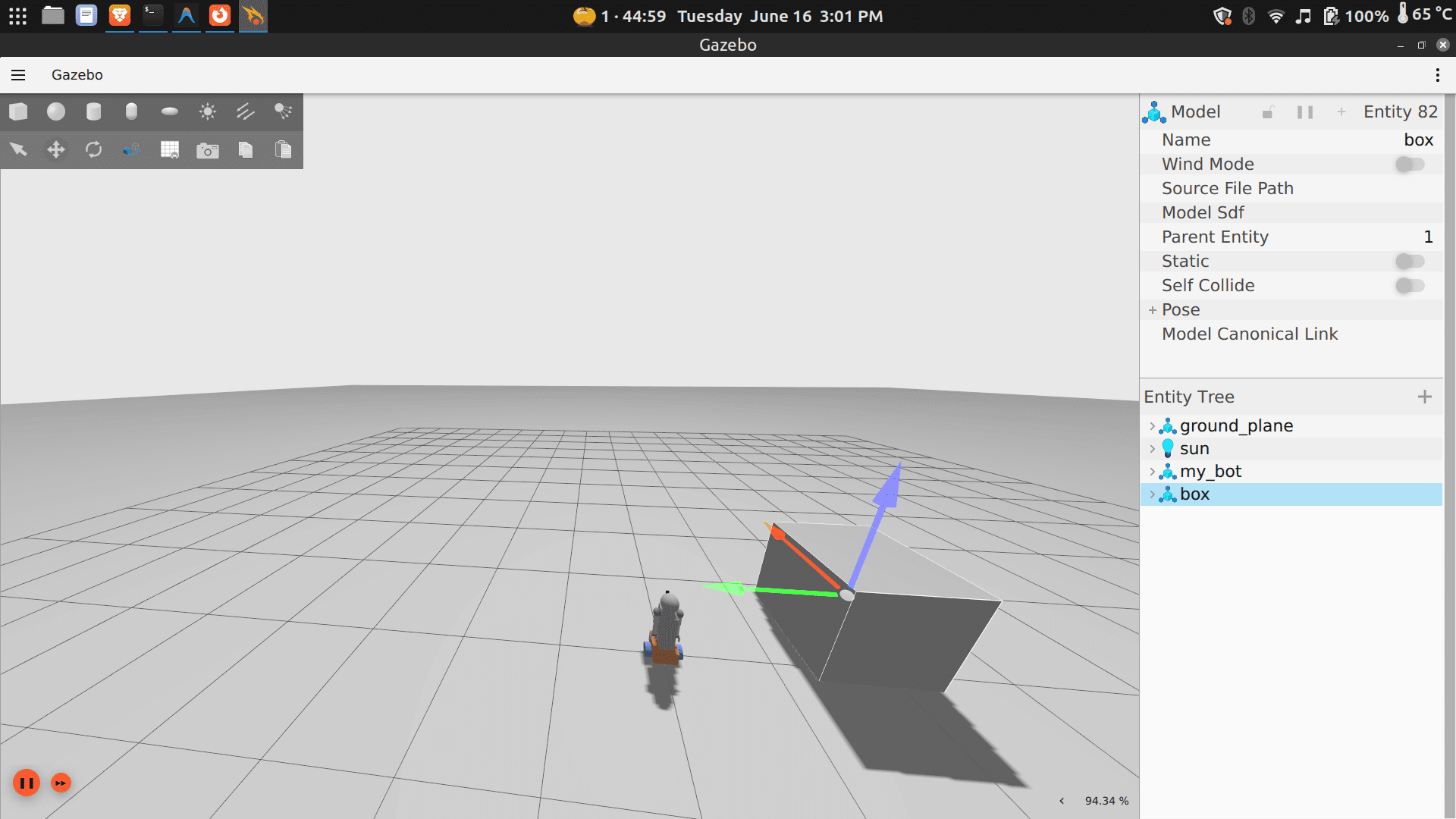
The easiest way to create a simple world is to open Gazebo and spend a few minutes exploring the interface — use the toolbar to insert shapes (boxes make great walls, cylinders work well as pillars), drag them into position, resize and rotate until you have something that resembles a navigable space. When you’re happy, go to File → Save World As and Gazebo writes the SDF for you.
Move the saved file into the worlds/ folder of your workspace:
bonicbot-a2-ros/
└── worlds/
    └── office_small.sdf    ← your saved world goes here
Working inside a Docker container? Copy the file in from your host machine using
docker cp:docker cp office_small.sdf <container_name>:/root/dev_ws/src/my_bot/worlds/
Next time you want to use this world, skip the rebuild — just launch it directly:
ros2 launch my_bot robot_system.launch.py use_sim_time:=true world:=office_small.sdfReplace
office_small.sdfwith whatever you named your file.
Option 2 — Use a World Built by Someone Else
You don’t have to build everything from scratch. The robotics community actively shares ready-made simulation environments through Gazebo Fuel — a public library of worlds and models you can download and use immediately.
Gazebo Fuel has environments ranging from simple rooms to full warehouses, hospitals, and outdoor terrains. Someone has likely already built something close to what you need.
Getting a world from Gazebo Fuel:
- Go to https://app.gazebosim.org/fuel/worlds
- Browse or search for an environment that fits your use case
- A good starting point is
tugbot_depot— a large warehouse well-suited for navigation testing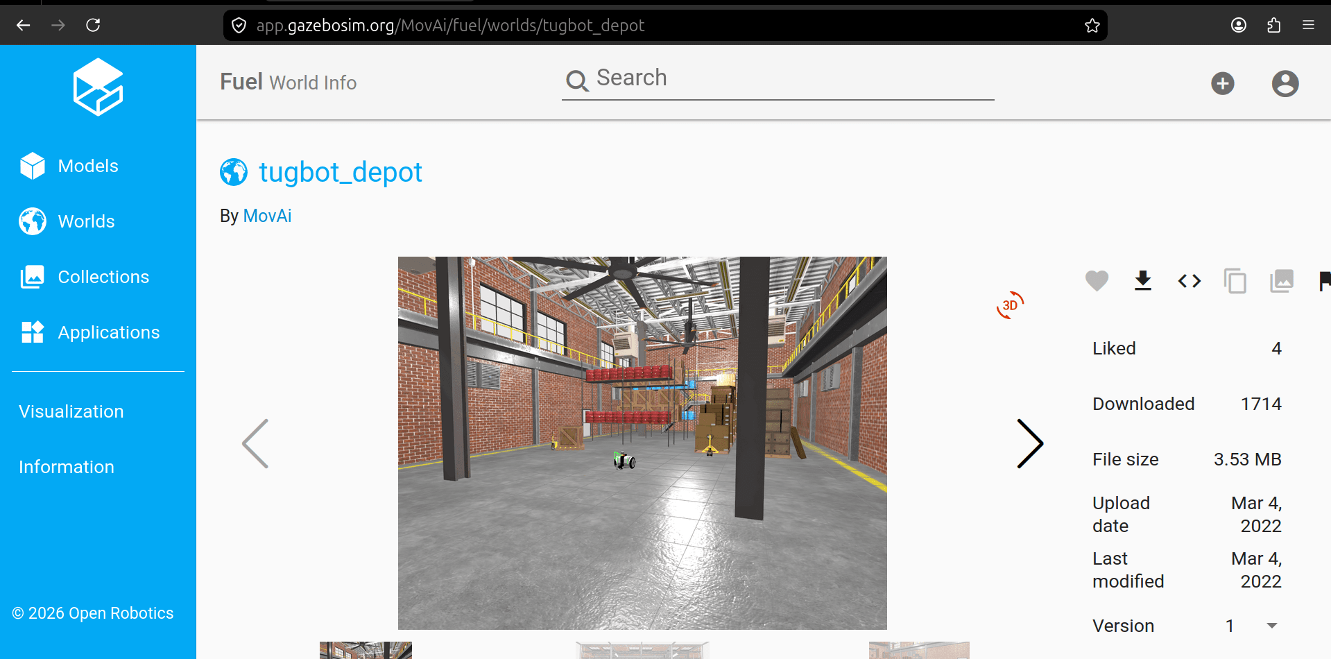
- Download the ZIP archive and extract it
- Save the
.sdffile and place it in yourworlds/folder
bonicbot-a2-ros/
└── worlds/
└── tugbot_depot.sdf ← your saved world goes here- Then launch the robot in this world:
cd ~/dev_ws
ros2 launch my_bot robot_system.launch.py use_sim_time:=true world:=tugbot_depot.sdf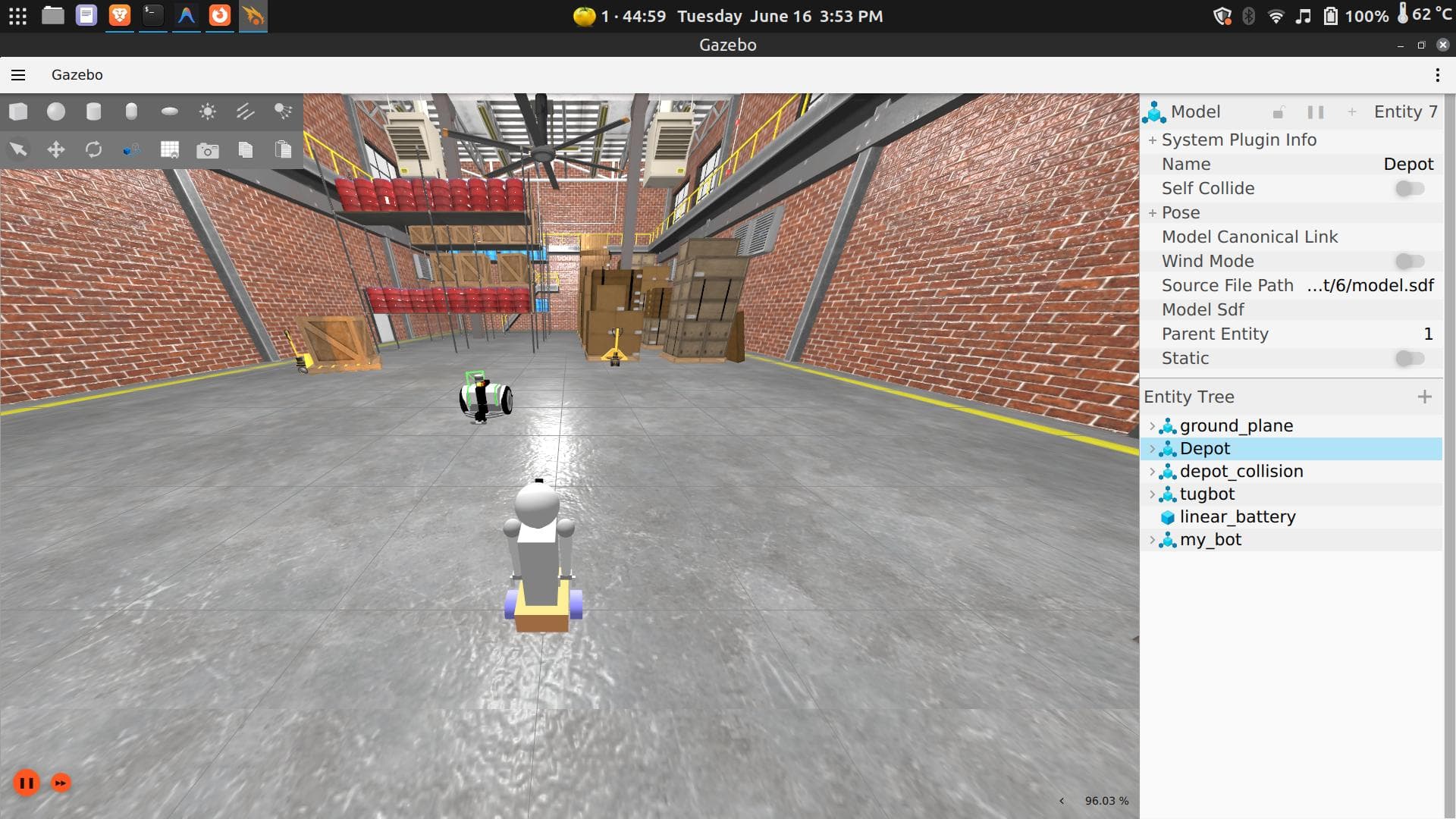
⚙️ Advanced — How the World You Just Downloaded Was Actually Made 🏗️
You have already downloaded a world from Gazebo Fuel, launched it in Gazebo, and driven a robot through it. What you may not have thought about is where that world came from in the first place — who made it, and how.
Every world on Gazebo Fuel, including tugbot_depot, was created by a developer or team who followed a deliberate, structured workflow before uploading it for the community to use. This section walks through that workflow so you can see exactly what happened behind the scenes.
Fuel Is a Community Repository
Think of Gazebo Fuel the same way you might think of GitHub. It is a place where developers publish finished work — in this case, simulation worlds and robot models — so that other people can discover and reuse them without starting from scratch.
When you downloaded tugbot_depot, you were not just grabbing a single file. You were receiving the final, packaged output of a significant amount of design and engineering work that someone completed and then chose to share publicly.
Step 1 — Designing the Environment
Before a single file was written, the person who created tugbot_depot made decisions about what kind of environment they wanted to simulate. In this case, a warehouse-style depot with shelving units, open floor space, and clear navigation lanes — conditions suitable for testing a logistics robot like the Tugbot.
This design phase is conceptual. It answers questions like: What are the dimensions of the space? What obstacles should exist? What behaviour should the robot be able to demonstrate or be challenged by? The answers to those questions drive everything that follows.
Step 2 — Building the 3D Models
Everything visible in the world — the warehouse walls, the shelving units, the floor markings, the structural columns — started as a 3D model created in modelling software such as Blender or FreeCAD, or exported from a CAD tool.
Each object was typically built in two versions:
- Visual model — the detailed version with geometry and textures that the rendering engine displays. This is what you see when you look around the depot in Gazebo.
- Collision model — a simplified version used only for physics calculations, such as detecting when the robot contacts a shelf. This is usually just a basic box or cylinder that approximates the shape of the object.
Keeping these separate is important for performance. Running physics against a fully detailed 3D mesh is expensive and will slow the simulation down significantly. The collision shape keeps things fast without affecting how the world looks.
If you browse inside the tugbot_depot package files, you will find mesh files (typically .obj or .dae format) that are exactly these geometry definitions — one set for visuals, one for collisions.
Step 3 — Describing the World in SDF
Once the individual models existed, the developer needed a way to tell Gazebo how to assemble them into a complete environment. This is done using a structured text file in a format called SDF (Simulation Description Format).
The SDF file for tugbot_depot is the single source of truth for the entire world. It specifies:
- which models exist in the environment and where each one is positioned
- the orientation and scale of every object
- physical properties such as mass and friction
- which robot to spawn, and at what starting position
Rather than placing objects manually through the GUI every time, the world is defined once in this file and can be reliably reconstructed from it. When you launch tugbot_depot, Gazebo reads that SDF file from top to bottom and builds the simulation from it — every shelf in exactly the right place, every wall at exactly the right height.
Step 4 — Adding Plugins and Dynamic Behaviour
A static scene of walls and shelves is functional, but real environments often have things that move. Plugins are small programs that attach to objects or to the world itself and give them dynamic behaviour. Common examples include:
- automatic doors that open as the robot approaches
- conveyor belts that carry objects along a path
- dynamic obstacles such as simulated people walking through the space
- sensor models that replicate the behaviour of specific hardware
Not every world uses plugins extensively, but the option exists whenever the simulation needs to go beyond a static scene.
Step 5 — Organising the Files
A finished simulation world is never a single file. The tugbot_depot package you downloaded contains a structured collection:
- The world SDF file — the blueprint that defines the full environment
- 3D mesh files — the geometry for each model (visual and collision versions)
- Texture image files — the images applied to surfaces to give them their appearance
- Model configuration files — metadata that tells Gazebo how to interpret each model and where to find its components
All of these live in dedicated folders, and the build system is configured to include them when the package is compiled. Gazebo also needs to know where to find the model files at runtime, which is configured through an environment variable called GAZEBO_MODEL_PATH.
Step 6 — Testing Locally, Then Publishing to Fuel
Once the world was assembled and working on the developer’s own machine, they uploaded the entire package to Gazebo Fuel. Fuel handled versioning, made it searchable, and made it available to anyone with a gz fuel download command.
That is precisely what you ran in the previous section. When you downloaded tugbot_depot from Gazebo Fuel, you were at the end of this entire pipeline — consuming the finished result of someone else’s design, modelling, SDF authoring, and testing work.
The Takeaway
The vast majority of robotics developers never need to follow this full workflow from scratch. They do exactly what you did — find a world on Fuel that closely matches their needs, download it, and use it. Building a custom world from the ground up only becomes necessary when an existing world does not match the real environment closely enough, and when that gap would meaningfully affect the robot’s performance.
For now, knowing that this workflow exists — and understanding that every world on Fuel is the product of it — gives you the context to make sense of what you are working with whenever you download and open one.
Option 3 — Generate a World Using an AI Assistant
You can describe your environment in plain English and ask an AI assistant to write the SDF world file for you. No modelling, no GUI work — just describe what you need and paste the result.
We’ve already done this for you. Here is a ready-to-use custom world file generated for this guide. Copy the XML and use it directly in your project:
📄 office_small.sdf — click to expand
<?xml version="1.0" ?>
<!--
  office_small.sdf
  A minimal realistic office room for testing my_bot navigation and perception.

  Layout (top-down, +X is right, +Y is up):
    - Room: 5m x 4m, centred at origin
    - Walls: 2.5m tall, 0.15m thick
    - Doorway: 1.0m wide opening in the south wall (Y = -2.0)
    - Desk: against the north wall
    - Chair: in front of the desk
    - Ceiling light: centred overhead

  Usage:
    ros2 launch my_bot robot_system.launch.py use_sim_time:=true world:=office_small.sdf
-->
<sdf version="1.9">
  <world name="office_small">

    <!-- ======================== Physics ======================== -->
    <physics name="1ms" type="ignored">
      <max_step_size>0.001</max_step_size>
      <real_time_factor>1.0</real_time_factor>
    </physics>

    <!-- ======================== System Plugins ======================== -->
    <plugin filename="gz-sim-physics-system"
            name="gz::sim::systems::Physics"/>
    <plugin filename="gz-sim-user-commands-system"
            name="gz::sim::systems::UserCommands"/>
    <plugin filename="gz-sim-scene-broadcaster-system"
            name="gz::sim::systems::SceneBroadcaster"/>
    <plugin filename="gz-sim-sensors-system"
            name="gz::sim::systems::Sensors">
      <render_engine>ogre2</render_engine>
    </plugin>
    <plugin filename="gz-sim-imu-system"
            name="gz::sim::systems::Imu"/>

    <!-- ======================== Scene ======================== -->
    <scene>
      <ambient>0.4 0.4 0.4 1</ambient>
      <background>0.7 0.7 0.7 1</background>
      <shadows>true</shadows>
    </scene>

    <gravity>0 0 -9.8</gravity>

    <!-- ======================== Lighting ======================== -->
    <!--
      Directional "sun" provides baseline illumination.
      Dimmed compared to outdoor worlds since this is an indoor room.
    -->
    <light type="directional" name="sun">
      <cast_shadows>true</cast_shadows>
      <pose>0 0 10 0 0 0</pose>
      <diffuse>0.5 0.5 0.5 1</diffuse>
      <specular>0.1 0.1 0.1 1</specular>
      <attenuation>
        <range>1000</range>
        <constant>0.9</constant>
        <linear>0.01</linear>
        <quadratic>0.001</quadratic>
      </attenuation>
      <direction>-0.5 0.1 -0.9</direction>
    </light>

    <!--
      Ceiling-mounted point light centred in the room at 2.4m height.
      Acts as the primary indoor illumination source.
      Warm white tone (0.95, 0.92, 0.85) simulates a standard office LED panel.
      Brightness tuned for camera-based perception (lidar is unaffected).
    -->
    <light type="point" name="ceiling_light">
      <pose>0 0 2.4 0 0 0</pose>
      <cast_shadows>true</cast_shadows>
      <diffuse>0.95 0.92 0.85 1</diffuse>
      <specular>0.3 0.3 0.3 1</specular>
      <intensity>1.5</intensity>
      <attenuation>
        <range>8</range>
        <constant>0.5</constant>
        <linear>0.1</linear>
        <quadratic>0.02</quadratic>
      </attenuation>
    </light>

    <!-- ======================== Ground Plane ======================== -->
    <model name="ground_plane">
      <static>true</static>
      <link name="link">
        <collision name="collision">
          <geometry>
            <plane>
              <normal>0 0 1</normal>
              <size>100 100</size>
            </plane>
          </geometry>
        </collision>
        <visual name="visual">
          <geometry>
            <plane>
              <normal>0 0 1</normal>
              <size>100 100</size>
            </plane>
          </geometry>
          <material>
            <ambient>0.5 0.5 0.5 1</ambient>
            <diffuse>0.5 0.5 0.5 1</diffuse>
            <specular>0.3 0.3 0.3 1</specular>
          </material>
        </visual>
      </link>
    </model>

    <!-- ======================== Floor ======================== -->
    <!--
      Separate floor surface sitting just above the ground plane.
      Represents the actual room floor with a warm light-oak wood tone.
      Friction set to realistic indoor floor values (mu=0.8).
      Size matches the room footprint: 5m x 4m.
    -->
    <model name="floor">
      <static>true</static>
      <pose>0 0 0.005 0 0 0</pose>
      <link name="link">
        <collision name="collision">
          <geometry>
            <box>
              <size>5.0 4.0 0.01</size>
            </box>
          </geometry>
          <surface>
            <friction>
              <ode>
                <mu>0.8</mu>
                <mu2>0.8</mu2>
              </ode>
            </friction>
          </surface>
        </collision>
        <visual name="visual">
          <geometry>
            <box>
              <size>5.0 4.0 0.01</size>
            </box>
          </geometry>
          <material>
            <!-- Light oak wood floor colour -->
            <ambient>0.55 0.42 0.30 1</ambient>
            <diffuse>0.60 0.45 0.32 1</diffuse>
            <specular>0.2 0.2 0.2 1</specular>
          </material>
        </visual>
      </link>
    </model>

    <!-- ======================== Walls ======================== -->
    <!--
      Room dimensions: 5.0m (X) x 4.0m (Y)
      Wall height: 2.5m   |   Wall thickness: 0.15m
      Origin at room centre.

      North wall: Y = +2.075     (full 5m span)
      East wall:  X = +2.575     (full 4.15m span, corner-to-corner)
      West wall:  X = -2.575     (full 4.15m span, corner-to-corner)
      South wall: Y = -2.075     (split for 1.0m doorway centred at X=0)
    -->

    <!-- North wall -->
    <model name="wall_north">
      <static>true</static>
      <pose>0 2.075 1.25 0 0 0</pose>
      <link name="link">
        <collision name="collision">
          <geometry><box><size>5.0 0.15 2.5</size></box></geometry>
        </collision>
        <visual name="visual">
          <geometry><box><size>5.0 0.15 2.5</size></box></geometry>
          <material>
            <ambient>0.85 0.85 0.82 1</ambient>
            <diffuse>0.90 0.90 0.87 1</diffuse>
            <specular>0.1 0.1 0.1 1</specular>
          </material>
        </visual>
      </link>
    </model>

    <!-- East wall -->
    <model name="wall_east">
      <static>true</static>
      <pose>2.575 0 1.25 0 0 0</pose>
      <link name="link">
        <collision name="collision">
          <geometry><box><size>0.15 4.15 2.5</size></box></geometry>
        </collision>
        <visual name="visual">
          <geometry><box><size>0.15 4.15 2.5</size></box></geometry>
          <material>
            <ambient>0.85 0.85 0.82 1</ambient>
            <diffuse>0.90 0.90 0.87 1</diffuse>
            <specular>0.1 0.1 0.1 1</specular>
          </material>
        </visual>
      </link>
    </model>

    <!-- West wall -->
    <model name="wall_west">
      <static>true</static>
      <pose>-2.575 0 1.25 0 0 0</pose>
      <link name="link">
        <collision name="collision">
          <geometry><box><size>0.15 4.15 2.5</size></box></geometry>
        </collision>
        <visual name="visual">
          <geometry><box><size>0.15 4.15 2.5</size></box></geometry>
          <material>
            <ambient>0.85 0.85 0.82 1</ambient>
            <diffuse>0.90 0.90 0.87 1</diffuse>
            <specular>0.1 0.1 0.1 1</specular>
          </material>
        </visual>
      </link>
    </model>

    <!--
      South wall – split into two segments with a 1.0m doorway centred at X=0.
      Left segment:  X from -2.5 to -0.5  (2.0m wide, centre X = -1.5)
      Right segment: X from +0.5 to +2.5  (2.0m wide, centre X = +1.5)
    -->
    <model name="wall_south_left">
      <static>true</static>
      <pose>-1.5 -2.075 1.25 0 0 0</pose>
      <link name="link">
        <collision name="collision">
          <geometry><box><size>2.0 0.15 2.5</size></box></geometry>
        </collision>
        <visual name="visual">
          <geometry><box><size>2.0 0.15 2.5</size></box></geometry>
          <material>
            <ambient>0.85 0.85 0.82 1</ambient>
            <diffuse>0.90 0.90 0.87 1</diffuse>
            <specular>0.1 0.1 0.1 1</specular>
          </material>
        </visual>
      </link>
    </model>

    <model name="wall_south_right">
      <static>true</static>
      <pose>1.5 -2.075 1.25 0 0 0</pose>
      <link name="link">
        <collision name="collision">
          <geometry><box><size>2.0 0.15 2.5</size></box></geometry>
        </collision>
        <visual name="visual">
          <geometry><box><size>2.0 0.15 2.5</size></box></geometry>
          <material>
            <ambient>0.85 0.85 0.82 1</ambient>
            <diffuse>0.90 0.90 0.87 1</diffuse>
            <specular>0.1 0.1 0.1 1</specular>
          </material>
        </visual>
      </link>
    </model>

    <!-- ======================== Ceiling ======================== -->
    <!--
      Visual-only ceiling panel. No collision needed (robot cannot reach it).
      Closes the room visually from above.
    -->
    <model name="ceiling">
      <static>true</static>
      <pose>0 0 2.5 0 0 0</pose>
      <link name="link">
        <visual name="visual">
          <geometry>
            <box>
              <size>5.0 4.0 0.05</size>
            </box>
          </geometry>
          <material>
            <ambient>0.95 0.95 0.95 1</ambient>
            <diffuse>0.95 0.95 0.95 1</diffuse>
            <specular>0.05 0.05 0.05 1</specular>
          </material>
        </visual>
      </link>
    </model>

    <!-- ======================== Furniture ======================== -->

    <!--
      Office Desk (Gazebo Fuel – OpenRobotics/Desk).
      Placed against the north wall, rotated 180° to face into the room.
    -->
    <include>
      <uri>https://fuel.gazebosim.org/1.0/OpenRobotics/models/Desk</uri>
      <name>office_desk</name>
      <pose>0.5 1.4 0 0 0 3.14159</pose>
      <static>true</static>
    </include>

    <!--
      Office Chair (Gazebo Fuel – OpenRobotics/Office Chair).
      Positioned in front of the desk, facing towards it.
    -->
    <include>
      <uri>https://fuel.gazebosim.org/1.0/OpenRobotics/models/Office Chair</uri>
      <name>office_chair</name>
      <pose>0.5 0.3 0 0 0 0</pose>
      <static>true</static>
    </include>

  </world>
</sdf>
Save the world file as office_small.sdf and place it inside the worlds/ folder of your ROS 2 workspace:
~/dev_ws/
└── src/
    └── bonicbot-a2-ros/
        └── worlds/
            └── office_small.sdf    ← your saved world goes here
Working inside a Docker container? Copy the file in from your host machine instead:
docker cp office_small.sdf <container_name>:/root/dev_ws/src/my_bot/worlds/
Make sure your current working directory is your ROS 2 workspace:
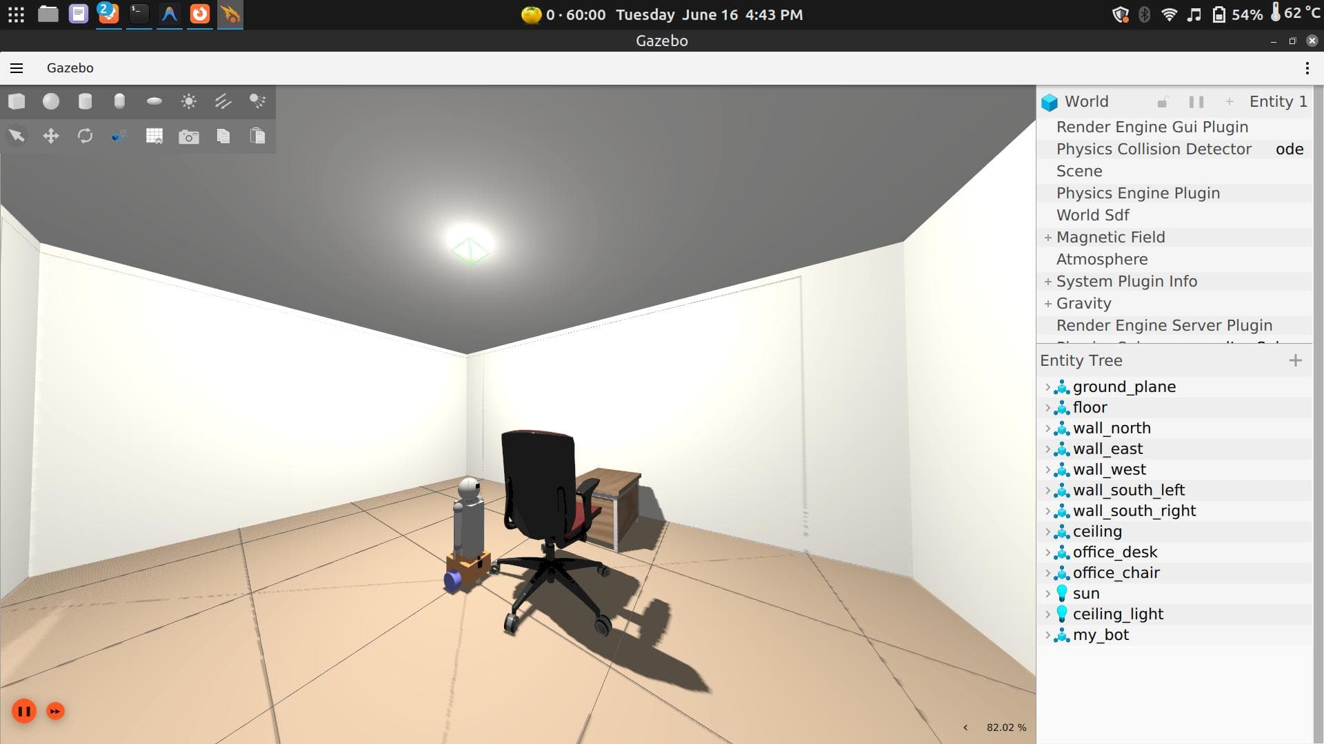
cd ~/dev_wsNow launch your robot inside your custom world:
ros2 launch my_bot robot_system.launch.py use_sim_time:=true world:=office_small.sdfReplace office_small.sdf with the name of your world file if you saved it with a different name.
Gazebo will now load your saved environment and spawn your robot inside it.
Troubleshooting — Clean Up Before Relaunching
If Gazebo fails to open, hangs, or spawns the robot incorrectly after a restart, stale background processes
are usually the cause. Pressing Ctrl+C or closing a terminal doesn’t always fully stop Gazebo, RViz, or the
ROS bridge — they linger and conflict with the next launch.
Before relaunching, run:
pkill -f ros2
pkill -f rosbridge
pkill -f rviz
pkill -f gz
pkill -f gazebo
Wait a moment, then relaunch normally.
Adding Individual Models to Existing Worlds
So far you’ve been launching complete world files. But you can also insert individual objects — people, furniture, equipment — into a world that’s already running, without stopping the simulation.
Download the Model
Download the Walking Person model from Gazebo Fuel:
https://app.gazebosim.org/Natzy/fuel/models/Walking person
Extract the downloaded archive to get the model files.
Set Up the Model Directory
Create a directory for the model inside your workspace and move the extracted files into it:
mkdir -p /root/dev_ws/models/person_walking
mv <your_extracted_files_here> /root/dev_ws/models/person_walking/
Once moved, your directory should look like this:
dev_ws/models/person_walking/
├── materials
│   └── textures
│       ├── eyebrow001.png
│       ├── eyebrow001-unmodified.png
│       ├── green_eye.png
│       ├── jeans01_normals.png
│       ├── jeans_basic_diffuse.png
│       ├── male02_diffuse_black.png
│       ├── male02_diffuse_black-unmodified.png
│       ├── teeth.png
│       ├── tshirt02_normals.png
│       ├── tshirt02_texture.png
│       └── young_lightskinned_male_diffuse.png
├── meshes
│   └── walking.dae
├── model.config
├── model.sdf
└── thumbnails
    ├── 1.png
    ├── 2.png
    ├── 3.png
    ├── 4.png
    └── 5.png
Why is the directory named
person_walking?This isn’t arbitrary — the directory name is intentionally chosen to match the model name referenced inside the SDF file. Gazebo models use relative paths and URI references that assume a specific directory structure. If you rename the folder, Gazebo can no longer resolve the mesh and texture paths inside the SDF, and the model will either fail to load or appear invisible. Keeping the directory name aligned with what the SDF expects avoids missing asset errors entirely.
Tell Gazebo Where to Find It
By default, Gazebo only searches a handful of built-in locations for models. If your model lives outside those paths — as it does here — Gazebo simply won’t find it, and the spawn command will fail silently or throw a path error.
The IGN_GAZEBO_RESOURCE_PATH environment variable tells Gazebo which additional directories to search when resolving model assets. You’ll set this in Terminal 1 before launching the world.
Spawn the Model Into the Running World
This takes two terminals — one to run the world, one to insert the model into it.
Terminal 1 — Launch the world
First, set the environment variable so Gazebo knows where to find your downloaded models:
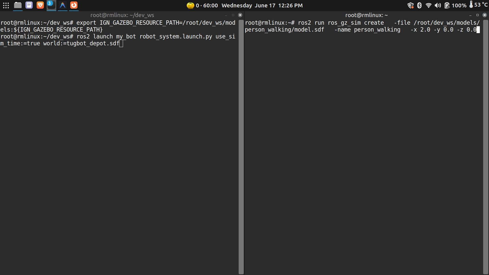
export IGN_GAZEBO_RESOURCE_PATH=/root/dev_ws/models:${IGN_GAZEBO_RESOURCE_PATH}Note: To avoid running this every time, add it to your
.bashrconce:echo 'export IGN_GAZEBO_RESOURCE_PATH=/root/dev_ws/models:${IGN_GAZEBO_RESOURCE_PATH}' >> ~/.bashrc source ~/.bashrc
Then launch the world:
cd ~/dev_ws
ros2 launch my_bot robot_system.launch.py use_sim_time:=true world:=tugbot_depot.sdf
Wait until the world is fully loaded in Gazebo before moving to Terminal 2.
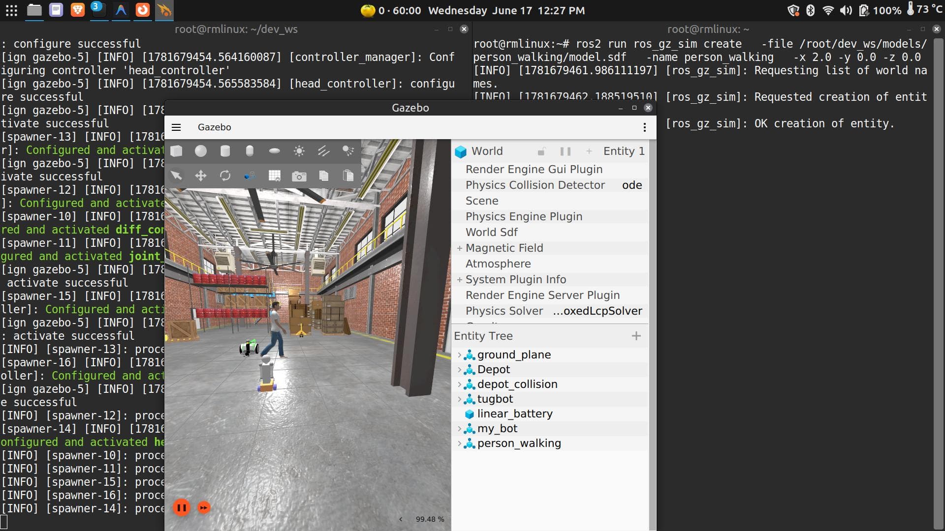
Terminal 2 — Insert the model
With the world already running, open a new terminal and spawn the Walking Person model into it:
ros2 run ros_gz_sim create \
  -file /root/dev_ws/models/person_walking/model.sdf \
  -name person_walking \
  -x 2.0 -y 0.0 -z 0.0
Here’s what each argument does:
-file— path to the model’s SDF file. Gazebo reads this to understand the model’s geometry, physics, and appearance.-name— the name this instance is given inside the running simulation. Used to identify, move, or remove the model later.-x,-y,-z— spawn position in the world, in metres. Adjust these to place the model where you want it.
A note on
-nameIt’s good practice to keep
-name person_walkingmatching the model name defined inside the SDF file. You can technically give it a different runtime name, but this can make debugging harder — especially when Gazebo logs or tools refer to the model by name and the names don’t match what you expect.
This is how you dynamically insert humans, furniture, and other objects into any running world — without restarting Gazebo and without modifying the world file itself.
Where to Go From Here
With custom worlds and dynamic model spawning in your toolkit, you have everything you need to start working on SLAM, autonomous navigation, obstacle avoidance, path planning, and sensor pipelines — all without touching the physical robot until you’re ready.
Go Deeper — Explore the Source
You’ve been running BonicBot A2’s ROS2 stack without looking inside it. Now open it up.
The ROS2 Package
git clone https://github.com/Autobonics/bonicbot-a2-ros.gitOpen it in your code editor and explore:
- How the robot description (URDF) defines the physical model
- How launch files wire nodes together
- How sensor drivers publish to topics
- How you can add your own nodes to the same system
This is a real, working ROS2 package — not a toy example. Reading it is one of the best ways to learn how production robotics software is structured.
The Python Library
git clone https://github.com/Autobonics/bonicbot-bridge.gitbonicbot-bridge is a Python library that lets you control and communicate with BonicBot A2 without writing raw ROS2 code. Install it with:
pip install bonicbot-bridgeThen open your editor and start experimenting:
from bonicbot_bridge import BonicBot

robot = BonicBot()
robot.move_forward(speed=0.3)
It’s a faster on-ramp for building applications — data logging, behaviour scripting, integrating sensors with your own logic — without needing to understand every ROS2 concept first.
🐍 Want to go further with
bonicbot-bridge? See the full Python SDK reference for the complete API, examples, and advanced usage.
Both repositories are open. Read them, fork them, modify them, break things. That’s how this is meant to be used.
What’s Coming
You’ve driven the robot, explored its data, and looked under the hood. The tutorials below pick up from here:
| Tutorial | What you’ll do |
|---|---|
| SLAM and Mapping | Drive through a space and generate a map in real time |
| Autonomous Navigation | Set a destination and let the robot find its own path |
| Writing ROS2 Nodes | Build your own publisher, subscriber, and service in Python |
| Sensor Pipelines | Process lidar and odometry data for your own applications |
| Working with bonicbot-bridge | Control the robot with Python in a few lines of code |